Rate of Change#
Functions are often visualized as a line on a graph, and this line shows how the value returned by the function changes based on changes in the input value.
Linear Rate of Change#
For example, imagine a function that returns the number of meters travelled by a cyclist based on the number of seconds that the cyclist has been cycling.
Here is such a function:
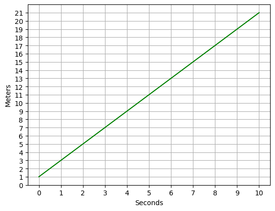
We can plot the output for this function for a period of 10 seconds like this:
%matplotlib inline

def q(x):
    return 2*x + 1

# Plot the function
import numpy as np
from matplotlib import pyplot as plt

# Create an array of x values from 0 to 10
x = np.array(range(0, 11))

# Set up the graph
plt.xlabel('Seconds')
plt.ylabel('Meters')
plt.xticks(range(0,11, 1))
plt.yticks(range(0, 22, 1))
plt.grid()

# Plot x against q(x)
plt.plot(x,q(x), color='green')

plt.show()

It’s clear from the graph that q is a linear function that describes a slope in which distance increases at a constant rate over time. In other words, the cyclist is travelling at a constant speed.
But what speed?
Speed, or more technically, velocity is a measure of change - it measures how the distance travelled changes over time (which is why we typically express it as a unit of distance per a unit of time, like miles-per-hour or meters-per-second). So we’re looking for a way to measure the change in the line created by the function.
The change in values along the line define its slope, which we know from a previous lesson is represented like this (refer 01-02 Linear Equations.ipynb and search for Slope):
We can calculate the slope of our function like this:
So we just need two ordered pairs of x and q(x) values from our line to apply this equation.
After 1 second, x is 1 and q(1) = 3.
After 10 seconds, x is 10 and q(10) = 21.
So we can meassure the rate of change like this:
This is the same as:
Which simplifies to:
So our rate of change is 2/1 or put another way, the cyclist is travelling at 2 meters-per-second.
Average Rate of Change#
OK, let’s look at another function that calculates distance travelled for a given number of seconds:
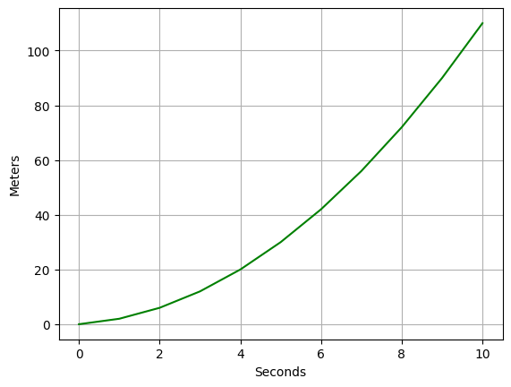
Let’s take a look at that using Python:
%matplotlib inline

def r(x):
    return x**2 + x

# Plot the function
import numpy as np
from matplotlib import pyplot as plt

# Create an array of x values from 0 to 10
x = np.array(range(0, 11))

# Set up the graph
plt.xlabel('Seconds')
plt.ylabel('Meters')
plt.grid()

# Plot x against r(x)
plt.plot(x,r(x), color='green')

plt.show()

This time, the function is not linear. It’s actually a quadratic function, and the line from 0 seconds to 10 seconds shows an exponential increase; in other words, the cyclist is accelerating.
Technically, acceleration itself is a measure of change in velocity over time; and velocity, as we’ve already discussed, is a measure of change in distance over time. So measuring accelleration is pretty complex, and requires differential calculus, which we’re going to cover shortly. In fact, even just measuring the velocity at a single point in time requires differential calculus; but we can use algebraic methods to calculate an average rate of velocity for a given period shown in the graph.
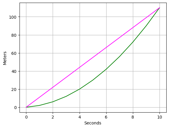
First, we need to define a secant line that joins two points in our exponential arc to create a straight slope. For example, a secant line for the entire 10 second time span would join the following two points:
0, r(0)
10, r(10)
Run the following Python code to visualize this line:
%matplotlib inline

def r(x):
    return (x)**2 + x

# Plot the function
import numpy as np
from matplotlib import pyplot as plt

# Create an array of x values from 0 to 10
x = np.array(range(0, 11))

# Create an array for the secant line
s = np.array([0,10])

# Set up the graph
plt.xlabel('Seconds')
plt.ylabel('Meters')
plt.grid()

# Plot x against r(x)
plt.plot(x,r(x), color='green')

# Plot the secant line
plt.plot(s,r(s), color='magenta')

plt.show()

Now, because the secant line is straight, we can apply the slope formula we used for a linear function to calculate the average velocity for the 10 second period:
At 0 seconds, x is 0 and r(0) = 0.
At 10 seconds, x is 10 and r(10) = 110.
So we can meassure the rate of change like this:
This is the same as:
Which simplifies to:
So our rate of change is 11/1 or put another way, the cyclist is travelling at an average velocity of 11 meters-per-second over the 10-second period.
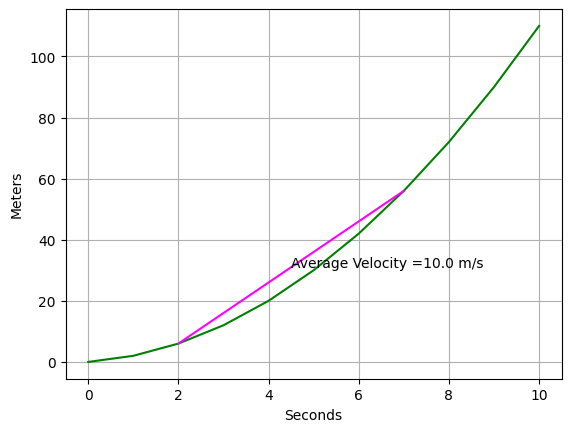
Of course, we can measure the average velocity between any two points on the exponential line. Use the following Python code to show the secant line for the period between 2 and 7 seconds, and calculate the average velocity for that period
%matplotlib inline

def r(x):
    return x**2 + x

# Plot the function
import numpy as np
from matplotlib import pyplot as plt

# Create an array of x values from 0 to 10
x = np.array(range(0, 11))

# Create an array for the secant line
s = np.array([2,7])

# Calculate rate of change
x1 = s[0]
x2 = s[-1]
y1 = r(x1)
y2 = r(x2)
a = (y2 - y1)/(x2 - x1)


# Set up the graph
plt.xlabel('Seconds')
plt.ylabel('Meters')
plt.grid()

# Plot x against r(x)
plt.plot(x,r(x), color='green')

# Plot the secant line
plt.plot(s,r(s), color='magenta')

plt.annotate('Average Velocity =' + str(a) + ' m/s',((x2+x1)/2, (y2+y1)/2))

plt.show()

