Softmax and Cross Entrophy Loss#
Softmax#
Softmax function, a wonderful activation function for classification problems that turns numbers aka logits into probabilities that sum to one. Softmax function outputs a vector that represents the probability distributions of a list of potential outcomes

In deep learning, the term logits layer is popularly used for the last neuron layer of neural network for classification task which produces raw prediction values as real numbers ranging from [-infinity, +infinity ]. — Wikipedia
Logits are the raw scores output by the last layer of a neural network. Before activation takes place.
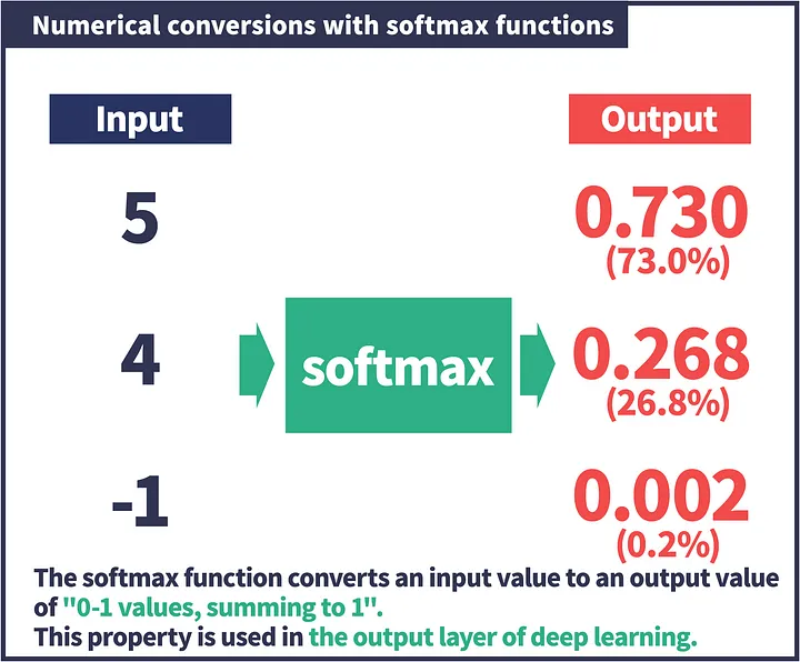
The above slide shows that Softmax function turns logits [5, 4, -1] into probabilities [0.730, 0.268, 0.002], and the probabilities sum to 1.
Softmax turn logits (numeric output of the last linear layer of a multi-class classification neural network) into probabilities by take the exponents of each output and then normalize each number by the sum of those exponents so the entire output vector adds up to one — all probabilities should add up to one. Softmax is frequently appended to the last layer of an image classification network such as those in CNN ( VGG16 for example) used in ImageNet competitions.
The softmax function \(h(x)\) mathematical representation consist of a temperature parameter \(\tau\) (temp_parameter) that controls the “sharpness” of the output probability distribution.
Mathematical Expression Explained#
Given:
\(x\), a feature vector from the dataset \(X\),
\(\theta\), a matrix of parameters where each row \(\theta_j\) represents the parameters for class \(j\),
\(\tau\), the temperature parameter that adjusts the distribution sharpness,
the softmax function \(h(x)\) is defined as:
This expression calculates the probability distribution over \(k\) classes for a given input vector \(x\), where:
The numerator \(e^{\theta_j \cdot x / \tau}\) is the exponentiated scaled dot product between the parameter vector for class \(j\) and the input vector \(x\), making the raw scores positive and scaling them according to \(\tau\).
The denominator is the sum of these exponentiated, scaled dot products for all classes, ensuring that the probabilities sum to 1.
n03an’s attempt#
If the above explanation isnt clear then understand that the last layer of a multi-class neural network would always be represented with scores accross \(k\) finite classes. And then you apply Softmax to show probabilities for these scores (all probabilities would sum to 1), out of which one of more class probability be activated (have higher values / probabilities). The goal is to classify into one confident class.
Example: In an image recognization problem with 3 classes as cat,dog and horse

For the first input image on the left, the first row of middle square represents last layer of neural network with 3 scores [5, 4, 2] accross 3 classses [cat, dog, horse], which is then fed into Softmax to calculate probabilities [0.71, 0.26, 0.04]. Its clear that the class cat is activated with higher probability of 0.71. Similarly for second image, the horse class is activated. BUT for the last image, both cat and dog have equal probability and this allows the model to respont “I am not sure” with an indication that it could be cat or dog.
Preventing numerical overflow#
Note: the terms \(e^{\theta_j \cdot x / \tau}\) may be very large or very small, due to the use of the exponential function. This can cause numerical or overflow errors. To deal with this, we can simply subtract some fixed amount \(c\) from each exponent to keep the resulting number from getting too large.
Why not just divide each logits by the sum of logits?#
Why do we need exponents? Logits is the logarithm of odds (wikipedia https://en.wikipedia.org/wiki/Logit) see the graph on the wiki page, it ranges from negative infinity to positive infinity. When logits are negative, adding it together does not give us the correct normalization. exponentiate logits turn them them zero or positive!
e**(100) = 2.6881171e+43
e**(-100) = 3.720076e-44 # a very small number
3.720076e-44 > 0 # still returns true
By the way, special number e exponents also makes the math easier later! Logarithm of products can be easily turned into sums for easy summation and derivative calculation. log(a*b)= log(a)+log(b)
Python Implementation#
To implement the softmax function as described for a dataset \(X\) and parameter matrix \(\theta\), you can use the following Python code:
import numpy as np
import mnist.utils as U

def compute_softmax_probabilities(X, theta, temp_parameter):
    # Compute the scaled dot product: (n, d) dot (k, d).T -> (n, k)
    scaled_scores = np.dot(X, theta.T) / temp_parameter

    # Prevent numerical overflow by subtracting the max score from each score
    scaled_scores -= np.max(scaled_scores, axis=1, keepdims=True)

    # Exponentiate the adjusted scores
    exp_scores = np.exp(scaled_scores)

    # Normalize the scores to get probabilities: (n, k)
    probabilities = exp_scores / np.sum(exp_scores, axis=1, keepdims=True)

    # Transpose to match the expected output shape (k, n)
    return probabilities.T
Explanation#
Compute Scaled Scores: Multiply the input matrix \(X\) by the transpose of the parameters matrix \(\theta\) and divide by the temperature parameter \(\tau\). This gives the scaled raw scores for each class and input.
Adjust for Numerical Stability: Subtract the maximum score from each scaled score within an input to prevent numerical overflow when exponentiating.
Exponentiate: Apply the exponential function to each adjusted score to ensure they are positive.
Normalize: Divide each exponentiated score by the sum of all exponentiated scores for that input. This step ensures that the probabilities for each input sum up to 1 across all classes.
Transpose: The resulting matrix is transposed to match the expected output shape \((k, n)\), where each entry \(H[j][i]\) represents the probability that input \(X[i]\) is labeled as class \(j\).
Binary cross-entrophy / log loss#
When we train classification models, we are most likely to define a loss function that describes how much out predicted values deviate from the true values. Then we will use gradient descent methods to adjust model parameters in order to lower the loss. It is a type of optimization problem, and also called backpropagation in deep learning.
Let’s start with 10 random points:
x = [-2.2, -1.4, -0.8, 0.2, 0.4, 0.8, 1.2, 2.2, 2.9, 4.6]

Now, let’s assign some colors to our points: red and green. These are our labels.

So, our classification problem is quite straightforward: given our feature x, we need to predict its label: red or green. Since this is a binary classification, we can also pose this problem as: “is the point green” or, even better, “what is the probability of the point being green”? Ideally, green points would have a probability of 1.0 (of being green), while red points would have a probability of 0.0 (of being green).
Now if we plot the points using sigmoid curve, representing the probability of a point being green for any given x . It looks like this:

i.e. for all the points belonging to the positive class (green), the probability would be

and for negative class (red)

or perhaps
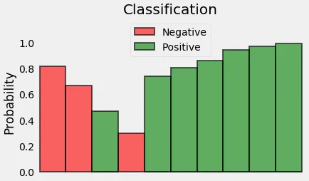
Since we’re trying to compute a loss, we need to penalize bad predictions. So, if the probability associated with the true class is 1.0, we need its loss to be zero. Conversely, if that probability is low, say, 0.01, we need its loss to be HUGE!
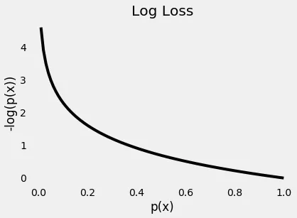
The plot below gives us a clear picture —as the predicted probability of the true class gets closer to zero, the loss increases exponentially
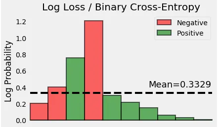
Let’s take the (negative) log of the probabilities — these are the corresponding losses of each and every point.
Finally, we compute the mean of all these losses.
from sklearn.linear_model import LogisticRegression
from sklearn.metrics import log_loss
import numpy as np

x = np.array([-2.2, -1.4, -.8, .2, .4, .8, 1.2, 2.2, 2.9, 4.6])
y = np.array([0.0, 0.0, 1.0, 0.0, 1.0, 1.0, 1.0, 1.0, 1.0, 1.0])

logr = LogisticRegression(solver='lbfgs')
logr.fit(x.reshape(-1, 1), y)

y_pred = logr.predict_proba(x.reshape(-1, 1))[:, 1].ravel()
loss = log_loss(y, y_pred)

print('x = {}'.format(x))
print('y = {}'.format(y))
print('p(y) = {}'.format(np.round(y_pred, 2)))
print('Log Loss (OR) Cross Entropy = {:.4f}'.format(loss))
x = [-2.2 -1.4 -0.8  0.2  0.4  0.8  1.2  2.2  2.9  4.6]
y = [0. 0. 1. 0. 1. 1. 1. 1. 1. 1.]
p(y) = [0.19 0.33 0.47 0.7  0.74 0.81 0.86 0.94 0.97 0.99]
Log Loss (OR) Cross Entropy = 0.3329
Distribution and Entrophy#
Let’s start with the distribution of our points. Since y represents the classes of our points (we have 3 red points and 7 green points), this is what its distribution, let’s call it q(y), looks like:
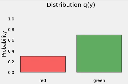
Entropy is a measure of the uncertainty associated with a given distribution q(y).
So if all our points were green then there is no uncertainty in distribution. So, entropy is zero!
On the other hand, what if we knew exactly half of the points were green and the other half, red? That’s the worst case scenario. We would have absolutely no edge on guessing the color of a point: it is totally random! For that case, entropy is given by \(log(2)\) (we have two classes (colors)— red or green — hence, 2). So, if we know the true distribution of a random variable, we can compute its entropy. But, what if we DON’T? Can we try to approximate the true distribution with some other distribution, say, p(y)
Log Loss (Binary Cross-Entropy Loss)#
The mathematical expression for log loss, also known as binary cross-entropy, for a set of observations is given by:
Where:
\(N\) is the total number of observations.
\(y_i\) is the actual label of the \(i\)-th observation, which can be 0 or 1 in binary classification.
\(p_i\) is the predicted probability of the \(i\)-th observation for being in class 1 (positive class).
\(\log\) is the natural logarithm.
This formula calculates the average loss per observation across all observations, penalizing the predicted probabilities based on how far they are from the actual labels. The goal in optimization is to minimize this loss, which corresponds to improving the accuracy of the predictions.
Since the log function has the property that when y is at 0, its log goes to -infinity; when y is at 1, its log is at 0, we can use it to model the loss pretty efficiently. For an instance with true label 0:
If the predicted value is 0, then the formula above will return a loss of 0.
If the predicted value is 0.5, then the formula above will return a loss of 0.69
If the predicted value is 0.99, then the formula above will return a loss of 4.6
from sklearn.linear_model import LogisticRegression
import numpy as np

# Given arrays
x = np.array([-2.2, -1.4, -.8, .2, .4, .8, 1.2, 2.2, 2.9, 4.6])
y = np.array([0.0, 0.0, 1.0, 0.0, 1.0, 1.0, 1.0, 1.0, 1.0, 1.0])

# Sigmoid function to convert logits to probabilities
def sigmoid(z):
    return 1 / (1 + np.exp(-z))

# Logistic regression model to predict probabilities
# Note, LR internally uses sigmoid function internally to model the probability that a given input belongs to the positive class
def logisticRegression(x, y):
    # Fit the logistic regression model
    logr = LogisticRegression(solver='lbfgs')
    logr.fit(x.reshape(-1, 1), y)
    # Predict probabilities
    p_lr = logr.predict_proba(x.reshape(-1, 1))[:, 1].ravel()
    return p_lr

# Convert logits x to probabilities p
p = sigmoid(x)
p_lr = logisticRegression(x, y)

# Calculate log loss
log_loss_sigmoid = -np.mean(y * np.log(p) + (1 - y) * np.log(1 - p))
log_loss_lr = -np.mean(y * np.log(p_lr) + (1 - y) * np.log(1 - p_lr))

print('p(y_lr) = {}'.format(np.round(p_lr, 2)))
print('p(y_sigmoid) = {}'.format(np.round(p, 2)))
print("Log Loss using Sigmoid:", log_loss_sigmoid)
print("Log Loss using LR:", log_loss_lr)
p(y_lr) = [0.19 0.33 0.47 0.7  0.74 0.81 0.86 0.94 0.97 0.99]
p(y_sigmoid) = [0.1  0.2  0.31 0.55 0.6  0.69 0.77 0.9  0.95 0.99]
Log Loss using Sigmoid: 0.3610786398744589
Log Loss using LR: 0.332939988498614
Cross-entrophy loss (Multi Class)#
After understanding the binary log loss, we can easily extend it to multi-class classification problems. Below \(J(\theta)\) is a generalized form of the cross-entropy loss function for multi class. It only sums the log of the probability when the instance class is \(j\), similar to the binary case, where there is always only part of the expression taken account of, and the others are just 0. The cost function \(J(\theta)\) uses softmax function for calculating probabilities and also includes a regularization term to prevent overfitting by penalizing large weights.
Mathematical Expression#
Given: \(n\) samples, each with \(d\) features and \(k\) possible classes
Where:
\(j\) is a single class from \(k\) possible classes. Similarly \(\theta\) represents parameter/weights for every d features in each class i.e. \(\theta _{j}\) represents \(d\) parameters/weights for class \(j\).
\(x^{(i)}\) denotes the feature vector of the \(i\)-th sample from \(n\) samples.
\(y^{(i)}\) is the actual class of the \(i\)-th sample.
\(\theta_j\) is the parameter vector for class \(j\).
\(\tau\) is the temperature parameter, adjusting the “sharpness” of the probability distribution.
\(\lambda\) is the regularization parameter controlling the extent of regularization.
\([[y^{(i)} == j]]\) is an indicator function that is 1 if \(y^{(i)}\) is class \(j\), and 0 otherwise.
The cost function consists of two parts:
Cross-Entropy Loss: The first term measures the prediction error. For each sample \(i\), it computes the log of the predicted probability for the true class \(y^{(i)}\), summed over all samples and classes. This term encourages the model to assign high probabilities to the correct classes.
Regularization Term: The second term is the regularization part, which sums the squares of all parameters in \(\theta\), scaled by \(\frac{\lambda}{2}\). This term discourages overly complex models by penalizing large weights.
Before we look at python code, lets understand One-Hot encoding
One-Hot Encoding (Multi Class Label’s)#
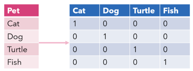
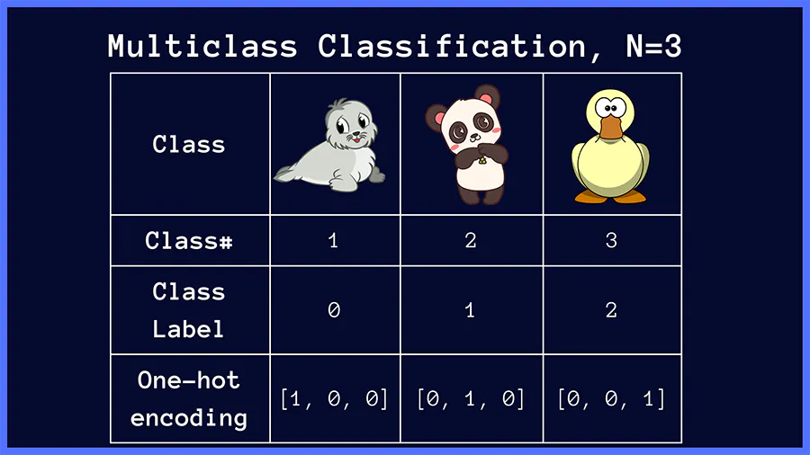
The One-Hot Encoding technique is crucial in machine learning and data processing, as it enables algorithms to efficiently handle and interpret categorical data, which is inherently non-numerical. This involves creating arrays where each category is represented by a distinct vector, with a ‘1’ in the position corresponding to the category and ‘0’s elsewhere.
Identify Unique Categories: Determine all the unique categories in your dataset.
Create a Binary Array: For each category, create an array where the length of the array is equal to the number of unique categories.
Fill Array By Category: The final step of creating a one-hot encoded array is a straightforward process. You start by initializing an array of zeros with dimensions that match the number of samples and the number of unique categories. Then, you iterate over your data, setting the appropriate element in each row to ‘1’ based on the category of that sample.
import numpy as np

# input vector
X = np.array(['cat', 'dog', 'fish', 'dog'])

# Step 1. Identify Unique Classes
# In addition also find their indices from input vector
classes, class_indices = np.unique(X, return_inverse=True)

n = X.size # number of samples
k = classes.size  # number of classes

# Create the one-hot encoded matrix
one_hot = np.zeros((n, k)) # Step 2: initialise a zero matrix of size (n, k)
one_hot[np.arange(n), class_indices] = 1 #Step 3. Encode Each Sample. Set the appropriate indices to 1

print(one_hot)

# Generating random data for testing
n, d, k = 100, 10, 3  # 100 samples, 10 features, 3 classes
X = np.random.randn(n, d)  # Random features
Y_one_hot = np.eye(k)[np.random.choice(k, n)]  # Random one-hot encoded labels
# np.eye(k) will create an identity matrix of size kxk. np.random.choice(k, n) will create random n size array with values from 0 to k-1.
# putting them together will generated a nxk matrix with each row would have 1 on the index based on random value from 0 to k-1
[[1. 0. 0.]
 [0. 1. 0.]
 [0. 0. 1.]
 [0. 1. 0.]]
Python Example for Cross-entrophy loss (Multi Class)#
Let’s implement this cost function in Python. Assume X is the feature matrix (n, d), Y is the one-hot encoded labels matrix (n, k), theta is the parameters matrix (k, d), tau is the temperature parameter, and lambda_ is the regularization parameter.
import numpy as np

def softmax(X, theta, temp_parameter):
    logits = np.dot(X, theta.T) / temp_parameter
    exp_logits = np.exp(logits - np.max(logits, axis=1, keepdims=True))
    probabilities = exp_logits / np.sum(exp_logits, axis=1, keepdims=True)
    return probabilities

def softmax_cost_function(X, Y, theta, tau, lambda_):
    # Compute the softmax probabilities
    probabilities = softmax(X, theta, tau)
    # Compute the cross-entropy loss
    cross_entropy_loss = -np.sum(Y * np.log(probabilities)) / X.shape[0]
    # Compute the regularization term
    regularization_term = (lambda_ / 2) * np.sum(theta ** 2)
    # Total cost
    total_cost = cross_entropy_loss + regularization_term
    return total_cost

n, d, k = 100, 10, 3  # 100 samples, 10 features, 3 classes
X = np.random.randn(n, d)  # Random features
Y = np.eye(k)[np.random.choice(k, n)]  # Random one-hot encoded labels
theta = np.random.randn(k, d)  # Random parameters
tau = 1.0
lambda_ = 0.1

cost = softmax_cost_function(X, Y, theta, tau, lambda_)
print(f"Softmax cost function value: {cost}")
Softmax cost function value: 3.450398446516297
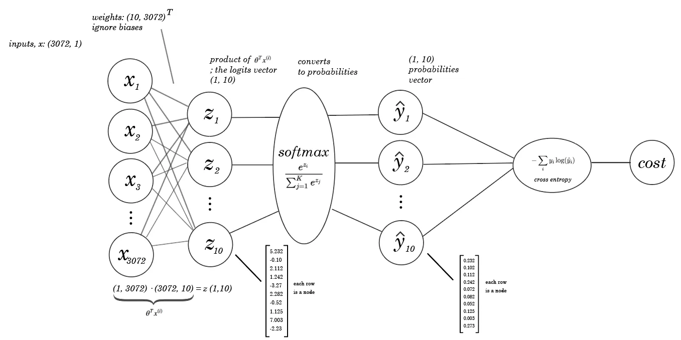
In above image classification example, if the target class is seal (class 1), the categorical cross-entropy loss is minimized when the network predicts a probability score close to 1 for the correct class (seal). This works similarly for the other target classes, panda and duck.
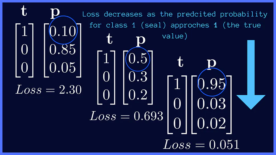
Here is another good visualization of how the Softmax and cost function is used on a neural network
Gradient Descent for Cross entrophy Loss and Softmax#
Lets recap
The softmax function is used in classification problems where the model needs to predict the probabilities that a given input belongs to each possible class. The output of the softmax function for a class is a value between 0 and 1, and the sum of these probabilities for all classes equals 1.
Mathematically, the softmax function for a class \(i\) given a vector \(x\) of raw class scores from the final layer of the model is defined as:
Where \(x_i\) is the score for class \(i\) and the denominator is the sum of the exponential scores for all \(j\) classes.
The simplest form of the cross-entropy loss function , which for a single example can be written as:
Where \(y_i\) is the actual distribution of classes (1 for the correct class, 0 for others) and \(\hat{y}_i\) is the predicted probability of each class.
We also learnt the cross entprophy loss function for \(n\) samples, each with \(d\) features and \(k\) possible classes (along with regularization term) can be written as
Gradient descent
is an optimization algorithm used to minimize some function by iteratively moving in the direction of steepest descent as defined by the negative of the gradient. In the context of softmax, the function we’re trying to minimize is the cost function, which measures the difference between the predicted probabilities and the actual class distributions.
The gradient of the loss function is \(\displaystyle \displaystyle \frac{\partial J(\theta )}{\partial \theta _ m}\) i.e. derivative of loss function by derative of the parameters \(\theta_m\)
Formula Breakdown#
\(\tau\): Temperature parameter that controls the “sharpness” of the softmax probabilities. A higher \(\tau\) makes the probabilities closer to uniform (softer), while a lower \(\tau\) makes the distribution more peaked.
\(n\): Number of training examples.
\(x^{(i)}\): Feature vector of the \(i\)-th training example.
\(y^{(i)}\): Actual label of the \(i\)-th training example.
\(m\): A particular class label out of \(k\) possible classes.
\([[y^{(i)} == m]]\): Indicator function that is 1 if \(y^{(i)}\) is equal to \(m\), and 0 otherwise.
\(p(y^{(i)} = m | x^{(i)}, \theta)\): Probability that the \(i\)-th example belongs to class \(m\), as predicted by the model parameterized by \(\theta\).
\(\lambda\): Regularization constant that controls the amount of regularization. Regularization helps prevent overfitting by penalizing large values of the parameters.
\(\theta_m\): Parameters associated with class \(m\).
Understanding the Gradient#
The formula consists of two main parts:
Gradient of the Loss Term: \(-\frac{1}{\tau n} \sum _{i = 1} ^{n} [x^{(i)}([[y^{(i)} == m]] - p(y^{(i)} = m | x^{(i)}, \theta ))]\)
This part computes the gradient of the loss function with respect to the parameters \(\theta_m\). The loss function measures the discrepancy between the actual labels and the predictions made by the model. The gradient points in the direction of the steepest increase in the loss function, and we subtract a fraction of this gradient (scaled by the learning rate) from \(\theta_m\) to update the parameters in the direction that minimally decreases the loss.
Gradient of the Regularization Term: \(\lambda \theta _m\)
This part represents the gradient of the regularization term with respect to \(\theta_m\). Adding this term to the gradient update discourages the parameters from growing too large, which helps prevent overfitting.
Python Example#
import matplotlib.pyplot as plt
import scipy.sparse as sparse

def run_gradient_descent_iteration(X, Y, theta, alpha, lambda_factor, temp_parameter):
    """
    Runs one step of batch gradient descent

    Args:
        X - (n, d) NumPy array (n datapoints each with d features)
        Y - (n, ) NumPy array containing the labels (a number from 0-9) for each
            data point
        theta - (k, d) NumPy array, where row j represents the parameters of our
                model for label j
        alpha - the learning rate (scalar)
        lambda_factor - the regularization constant (scalar)
        temp_parameter - the temperature parameter of softmax function (scalar)

    Returns:
        theta - (k, d) NumPy array that is the final value of parameters theta
    """
    #YOUR CODE HERE
    num_examples = X.shape[0]
    num_labels = theta.shape[0]
    itemp = 1. / (temp_parameter * num_examples)
    probabilities = compute_softmax_probabilities(X, theta, temp_parameter)

    """
        M[i][j] = 1 if y^(j) = i and 0 otherwise.
        M is a matrix of size (num_labels, num_examples) where each column is a one-hot encoded vector

        For example, if we have 3 classes and 4 examples, and the labels are [0, 1, 2, 1], then M would be:
        Coords	Values
        (0, 0)	1
        (1, 1)	1
        (2, 2)	1
        (1, 3)	1

        Note sparse matrix in COOrdinate format are used to store data efficiently when the matrix contains a lot of zeros...toarray() would convert it to one-hot encoded vector

        [[1 0 0 0]
        [0 1 0 1]
        [0 0 1 0]]
    """
    M = sparse.coo_matrix(([1] * num_examples, (Y, range(num_examples))),
                          shape=(num_labels, num_examples)).toarray()

    # X . (M - probabilities)
    graident_of_loss = np.dot(M - probabilities, X)
    graident_of_loss *= -itemp

    graident_of_regularized_term = lambda_factor * theta

    return theta - alpha * (graident_of_loss + graident_of_regularized_term)

# Example feature matrix (4 examples, 3 features each)
X = np.array([[1, 2, 3], [4, 5, 6], [7, 8, 9], [10, 11, 12]])
# Example labels (4 examples, 1 label each)
Y = np.array([0, 1, 2, 1])
# Initial parameters (3 classes, 3 features each)
theta = np.zeros((3, 3))
# Learning rate
alpha = 0.01
# Regularization constant
lambda_factor = 0.1
# Temperature parameter
temp_parameter = 1.0
# Running one iteration of gradient descent
theta_updated = run_gradient_descent_iteration(X, Y, theta, alpha, lambda_factor, temp_parameter)
print(theta_updated)
[[-0.01583333 -0.01666667 -0.0175    ]
 [ 0.01666667  0.01833333  0.02      ]
 [-0.00083333 -0.00166667 -0.0025    ]]
Temperature#
The concept of “temperature” in the context of applying the softmax function, especially in tasks like classification on the MNIST dataset, is a way to control the sharpness of the output probability distribution.
High Temperature ((T >= 1)): Increases the temperature value to make the softmax output more uniform (i.e., probabilities closer to each other). This can be useful for encouraging exploration in models or for making the model less confident in its predictions.
Low Temperature ((T < 1)): Decreases the temperature to make the softmax output sharper, with higher probabilities assigned to logits with larger values, making the model more confident in its predictions.
A lower temperature might be used when you’re confident about the model’s training and want to boost the prediction certainty, while a higher temperature might be useful in early training stages or when the model is overfitting by being too confident in its predictions.
Below Python code runs on MNIST dataset and computes test error at varing temperature
import utils as U
import part1.softmax as S

def run_softmax_on_MNIST(temp_parameter=1):
    """
    Trains softmax, classifies test data, computes test error, and plots cost function

    Runs softmax_regression on the MNIST training set and computes the test error using
    the test set. It uses the following values for parameters:
    alpha = 0.3
    lambda = 1e-4
    num_iterations = 150

    Saves the final theta to ./theta.pkl.gz

    Returns:
        Final test error
    """
    train_x, train_y, test_x, test_y = U.get_MNIST_data('Datasets/mnist.pkl.gz')
    theta, cost_function_history = S.softmax_regression(train_x, train_y, temp_parameter, alpha=0.3, lambda_factor=1.0e-4, k=10, num_iterations=150)
    S.plot_cost_function_over_time(cost_function_history)
    test_error = S.compute_test_error(test_x, test_y, theta, temp_parameter)
    # Save the model parameters theta obtained from calling softmax_regression to disk.
    # write_pickle_data(theta, "./theta.pkl.gz")
    # TODO: add your code here for the "Using the Current Model" question in tab 6.
    #      and print the test_error_mod3
    return test_error


print('softmax test_error=', run_softmax_on_MNIST(temp_parameter=0.5))
print('softmax test_error=', run_softmax_on_MNIST(temp_parameter=1.0))
print('softmax test_error=', run_softmax_on_MNIST(temp_parameter=2.0))
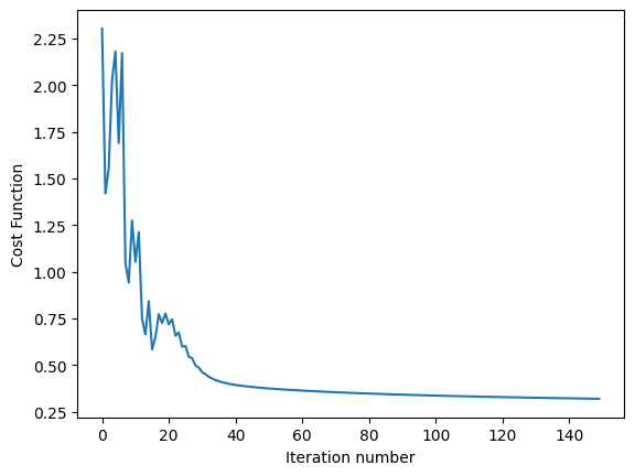
softmax test_error= 0.08399999999999996
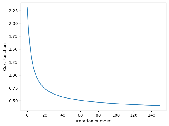
softmax test_error= 0.10050000000000003
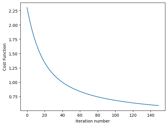
softmax test_error= 0.1261
