Nonlinear Classification

Nonlinear Classification#

We can use linear classifiers to make non-linear predictions. The easiest way to do this is to first map all the examples $x\in \mathbb {R}^ d$ to different feature vectors $\phi (x)\in \mathbb {R}^ p$ where typically $p$ is much larger than $d$. We would then simply use a linear classifier on the new (higher dimensional) feature vectors, pretending that they were the original input vectors. As a result, all the linear classifiers we have learned remain applicable, yet produce non-linear classifiers in the original coordinates.

There are many ways to create such feature vectors. One common way is to use polynomial terms of the original coordinates as the components of the feature vectors.

Higher Order Feature Vector#

Higher Order Feature Vectors are a technique used in machine learning to capture non-linear relationships between features and the target variable by introducing polynomial terms and interactions between features. This approach is particularly useful when the relationship between the input variables (features) and the output variable is not linear, and a linear model (like linear regression) cannot capture the complexity of the data.

Here’s a breakdown of the concept:

Basic Idea#

Linear Models: Traditional linear models predict the outcome based on a linear combination of input features. For example, in a simple linear regression, the predicted outcome $y$ is modeled as $y = \theta_0 + \theta_1x_1 + \theta_2x_2 + ... + \theta_nx_n$, where $x_1, x_2, ..., x_n$ are the features, and $\theta_0, \theta_1, ..., \theta_n$ are the model parameters.
Limitation: Linear models are limited in their ability to handle complex, non-linear relationships between the features and the target variable.

Higher Order Features#

Polynomial Features: To capture non-linear relationships, we can extend our feature set with polynomial terms. For example, if we have a single feature $x$, we can create additional features like $x^2, x^3, ..., x^d$, where $d$ is the degree of the polynomial. This allows the model to fit more complex patterns in the data.
Interaction Features: Besides polynomial terms, we can also include interaction terms between different features. For instance, if we have two features $x_1$ and $x_2$, we can include a feature representing their interaction $x_1 \times x_2$. This helps in capturing the effect of the interaction between variables on the target variable.

Implementation#

Feature Vector Expansion: The process involves expanding the original feature vector to include these higher order and interaction terms. For example, for two features $x_1$ and $x_2$, and using up to second-degree polynomials, the expanded feature vector might look like $[1, x_1, x_2, x_1^2, x_1x_2, x_2^2]$.
Model Training: After expanding the feature set, a linear model can be trained on this enhanced feature set. Despite the model being linear in parameters, the inclusion of higher order features allows it to capture non-linear relationships in the data.

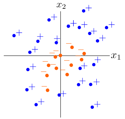
Given the training examples with $\displaystyle x=\left[x_1^{(t)},x_2^{(t)}\right]\in \mathbb {R}^2$ above, where a boundary between the positively-labeled examples and the negatively-labeled examples is an ellipse

Higher Order Feature vector can be written as:

\[ \displaystyle \phi (x)=[x_1,\, x_2,\, x_1x_2,\, x_1^2,\, x_2^2]^ T \]

Considerations#

Overfitting: Introducing higher order features increases the model’s complexity, which can lead to overfitting. Regularization techniques like Ridge or Lasso regression are often used alongside to mitigate this risk.
Feature Space Explosion: The number of higher order and interaction terms can grow quickly with the number of original features and the degree of the polynomial, leading to a high-dimensional feature space. It’s important to select the degree of the polynomial and the interactions judiciously.

Higher Order Feature Vectors are a powerful way to extend linear models to address non-linear problems, making them more flexible and applicable to a wider range of datasets.

Counting dimensions of feature vectors#

The dimension of a feature vector refers to the number of features (or attributes) that the vector contains.

Question: Let $x \in \mathbf{R}^{150},$ i.e. $x = \big [ x_1, x_2, ..., x_{150} \big ]^ T$ where $x_ i$ is the i-th component of x. Let $\phi (x)$ be an order $3$ polynomial feature vector.

\[ \displaystyle \phi (x) = \big [\underbrace{x_1, ..., x_ i, ..., x_{150}}_{{\color{blue}{\text {deg 1}}} }, \underbrace{x_1^2, x_1x_2, ..., x_ i x_ j,...{x_{150}}^2}_{{\color{blue}{\text {deg 2}}} }, \underbrace{{x_1}^3, {x_1}^2 x_2,..., x_ i x_ j x_ k, ..., {x_{150}}^3}_{{\color{blue}{\text {deg 3}}} } \big ]\qquad \]

\[ \text {where }\, 1\leq i\leq j\leq k\leq 150. \]

What is the dimension of the space that $\phi (x)$ lives in? That is, $\phi (x)\in \mathbb {R}^ d$ for what $d$?

Hint: The number of ways to select a multiset of $k$ non-unique items from total is $$ \displaystyle {n + k - 1 \choose k} $$

Given a feature vector $x$ with 150 components and considering polynomial terms up to degree 3, we can calculate the total number of terms as follows:

Degree 1 terms: 150 terms (one for each feature). $$\displaystyle {150 + 1 - 1 \choose 1}$$
Degree 2 terms: This includes all combinations of the features taken two at a time (including squares). $$\displaystyle {150 + 2 - 1 \choose 2}$$
Degree 3 terms: This includes all combinations of the features taken three at a time. $$\displaystyle {150 + 3 - 1 \choose 3}$$

Let’s compute these values using Python.

import math

# Number of features
n = 150

# Function to compute binomial coefficient
def binomial_coefficient(n, k):
    return math.comb(n, k)

# Degree 1 terms
deg1_terms = binomial_coefficient(n, 1)

# Degree 2 terms
deg2_terms = binomial_coefficient(n + 1, 2)

# Degree 3 terms
deg3_terms = binomial_coefficient(n + 2, 3)

# Total terms
total_terms = deg1_terms + deg2_terms + deg3_terms

print(f"The dimension of the space that phi(x) lives in is: d = {total_terms}")

The dimension of the space that phi(x) lives in is: d = 585275