Loss Function#
Machine learning is nothing but an optimisation problem. Researchers use an algebraic acme called Losses in order to optimise the machine learning space defined by a specific use case. A “Loss” can be seen as a distance between the true values of the problem and the values predicted by the model. The greater the loss is, the more huge the errors you made on the data. Most of the performance evaluation metrics such as accuracy, precision, recall, f1 score etc are an indirect derivation of the Loss functions. There are a lot of loss functions implemented by the researchers like-
For Regression problems- Mean Squared Error, Mean of Absolute Error, Huber Loss, Log Cosh Loss, Quantile Loss etc.
For Binary classification problems - Binary Cross Entropy Loss, Hinge Loss etc.
For Multi classification problems - Multi-Class Cross Entropy Loss, KL- Divergence
Hinge Loss#
Hinge loss is a function popularly used in support vector machine algorithms to measure the distance of data points from the decision boundary. This helps approximate the possibility of incorrect predictions and evaluate the model’s performance.
The support vector machine (SVM) is a supervised machine learning algorithm that is popularly used for predicting the category of labelled data points. e.g. Predicting whether a person is male or female OR Predicting whether the fruit is an apple or orange OR Predicting whether a student will pass or fail the exams etc etc.
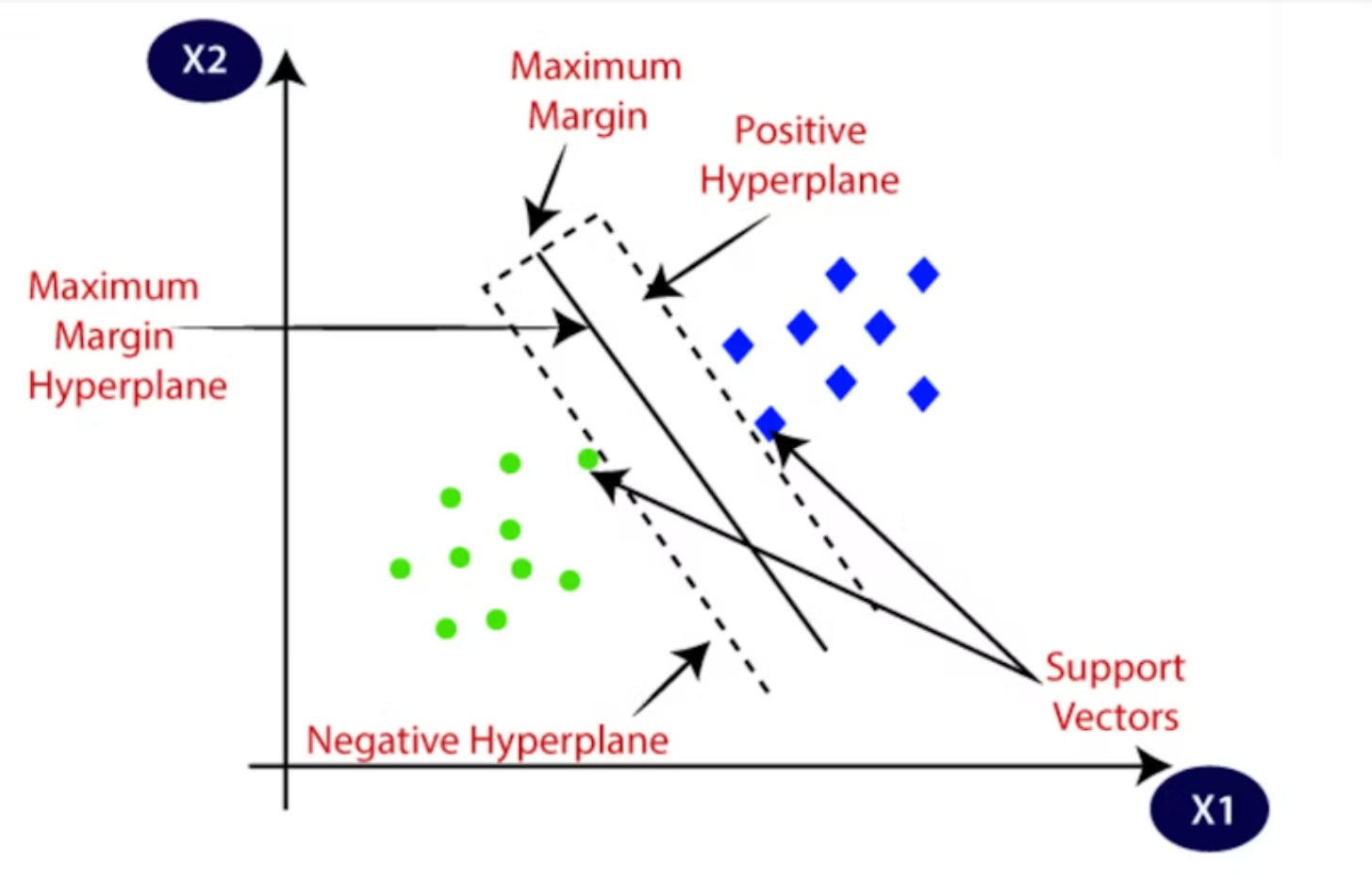
SVM uses an imaginary plane that can travel across multiple dimensions for its prediction purpose. These imaginary planes which can travel through multiple dimensions are called hyperplanes. It is very difficult to imagine higher dimensions using human brains since our brain is naturally capable to visualize only up to 3 dimensions.
Lets take a classification problem to predict whether a student will pass or fail the examination

The Hyperplane is the decision boundary or maximum margin hyperplane. The distance from a data point to the decision boundary shows the strength of the predition.
Logically,
If the distance between the decision boundary and the data point is relatively large then it means that the model is somewhat confident about its prediction.
If the distance between the decision boundary and the data point is relatively low then it means that the model is less confident about its prediction.
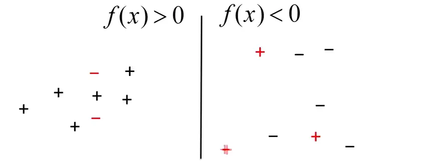
The points on the left side are correctly classified as positive and those on the right side are classified as negative. Misclassified points are marked in RED.

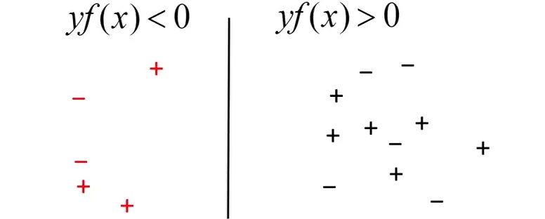
Now, we can try bringing all our misclassified points on one side of the decision boundary. Let’s call this ‘the ghetto’.


Mathematically, Hinge loss for a data point can be represented as : $\(L_h(y,f(x))=max(0,1–y∗f(x))\)$
yis the actual class (-1 or 1)f(x)is the output of the classifier for the datapoint
Loss Function OR Error Function#
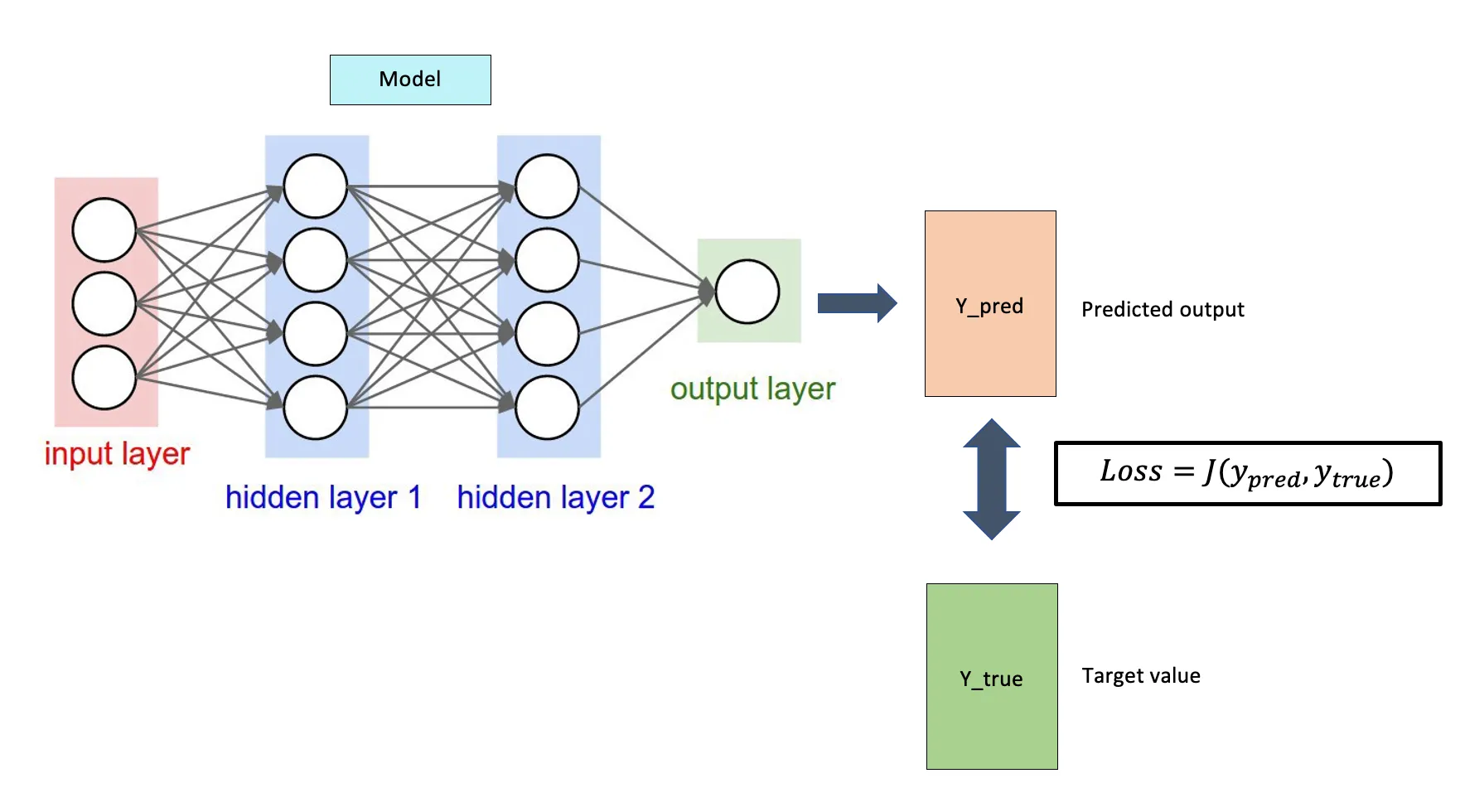
Are used to gauge the error between the prediction output and the provided target value. A loss function will determine the model’s performance by comparing the distance between the prediction output and the target values. Smaller loss means the model performs better in yielding predictions closer to the target values.
Given below neural network
Predicted output (y_pred)
Target value (y_true)

Regression Loss:
Mean Square Error or L2 Loss
Mean Absolute Error or L1 Loss
Huber Loss
Classification Loss:
Binary Classification:
Hinge Loss
Sigmoid Cross Entropy Loss
Weighted Cross Entropy Loss
Multi-Class Classification:
Softmax Cross Entropy Loss
Sparse Cross Entropy Loss
Cost Function#
Cost functions aggregate the difference for the entire training dataset
For a given hinge loss function (for each training example)
The cost function (for entire training set) would be sum of each training example loss, divided by number of examples to get average cost
Where
X is the feature matrix.
y is the target vector.
w is the weights vector.
b is the bias.
import numpy as np

def calculate_cost(X, y, w, b):
    m = len(y)
    total_cost = 0
    for i in range(m):
        hinge_loss = max(0, 1 - y[i] * (np.dot(w, X[i]) + b))
        print(f"Hinge Loss for vector {X[i]}, target {y[i]}: {hinge_loss}")
        total_cost += hinge_loss
    return total_cost / m

# Example usage:
X = np.array([[1, 1], [2, 3], [3, 5], [1, -1], [2, -2], [3, -4]])  # feature matrix
y = np.array([1, 1, 1, -1, -1, -1])  # target vector
w = np.array([0.0, 0.0])  # initial weights
b = 0.0  # initial bias
print(f"Total Cost: {calculate_cost(X, y, w, b)}")
Hinge Loss for vector [1 1], target 1: 1.0
Hinge Loss for vector [2 3], target 1: 1.0
Hinge Loss for vector [3 5], target 1: 1.0
Hinge Loss for vector [ 1 -1], target -1: 1.0
Hinge Loss for vector [ 2 -2], target -1: 1.0
Hinge Loss for vector [ 3 -4], target -1: 1.0
Total Cost: 1.0
