Classifiers#
Training data can be graphically depicted on a (hyper)plane. Classifiers are mappings that take feature vectors as input and produce labels as output. A common kind of classifier is the linear classifier, which linearly divides space(the (hyper)plane where training data lies) into two. Given a point \(x\) in the space, the classifier \(h\) outputs \(h(x) = 1\) or \(h(x) = -1\), depending on where the point \(x\) exists in among the two linearly divided spaces.
Here is an example of multiple classifer in (hyper)plane
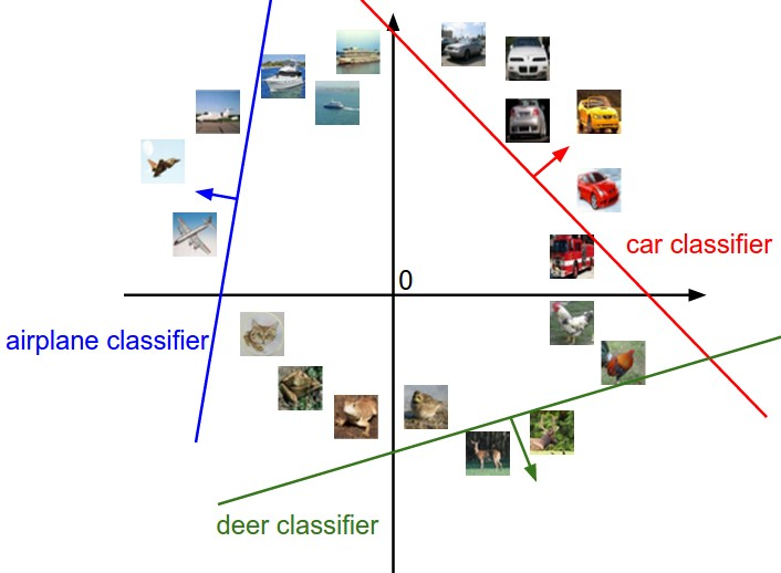
Here’s an example of a Python program that demonstrates a linear classifier using the scikit-learn library:
from sklearn.linear_model import LogisticRegression
from sklearn.model_selection import train_test_split
from sklearn.datasets import load_iris
import numpy as np

# Load the Iris dataset
iris = load_iris()
X = iris.data
y = iris.target

# Split the dataset into training and testing sets
X_train, X_test, y_train, y_test = train_test_split(X, y, test_size=0.2, random_state=42)

print("Training set size:", len(X_train))
print("Test set size:", len(X_test))
print("Features:", iris.feature_names)
print("Classes:", iris.target_names)

# Create a linear classifier model
classifier = LogisticRegression()

# Train the model using the training data
classifier.fit(X_train, y_train)

# Predict the classes for the test data
y_pred = classifier.predict(X_test)

# Evaluate the accuracy of the model
accuracy = classifier.score(X_test, y_test)
print("Accuracy:", accuracy)
Training set size: 120
Test set size: 30
Features: ['sepal length (cm)', 'sepal width (cm)', 'petal length (cm)', 'petal width (cm)']
Classes: ['setosa' 'versicolor' 'virginica']
Accuracy: 1.0
/Users/n03an/.pyenv/versions/3.11.5/lib/python3.11/site-packages/sklearn/linear_model/_logistic.py:460: ConvergenceWarning: lbfgs failed to converge (status=1):
STOP: TOTAL NO. of ITERATIONS REACHED LIMIT.

Increase the number of iterations (max_iter) or scale the data as shown in:
    https://scikit-learn.org/stable/modules/preprocessing.html
Please also refer to the documentation for alternative solver options:
    https://scikit-learn.org/stable/modules/linear_model.html#logistic-regression
  n_iter_i = _check_optimize_result(
In this example, we are using the Iris dataset, which is a popular dataset for classification tasks. We split the dataset into training and testing sets using the train_test_split function from scikit-learn. Then, we create a LogisticRegression classifier and train it using the training data. Finally, we use the trained model to predict the classes for the test data and evaluate the accuracy of the model
Hypothesis Space#
In machine learning, the “hypothesis space” refers to the set of all possible models that can be learned given a particular learning algorithm.
For example, if you’re using a linear regression algorithm, the hypothesis space includes all possible linear functions that can be created by the algorithm. If you’re using a decision tree algorithm, the hypothesis space includes all possible decision trees that can be created.
The learning algorithm searches within this hypothesis space to find the model that best fits the training data, according to some objective function or criterion (like minimizing the error between the model’s predictions and the actual values).
Classification and Regression#
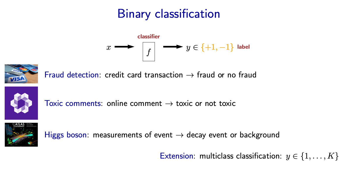
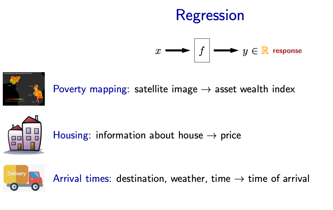
Classification maps feature vectors to categories. The number of categories need not be two - they can be as many as needed. Regression maps feature vectors to real numbers. There are other kinds of supervised learning as well.
Example Classification Problem: Come up with a classifier that classifies each news article into one of the following categories: politics, sports, entertainment.
Example Regression Problem: Estimate the price of bitcoin after 30 days
Concepts#
Feature Vector: A feature vector is an n-dimensional vector of numerical features that represent some object. In mathematical terms, if an object has n features, its feature vector x can be represented as \(x = [x1, x2, ..., xn]\)
Labels: Labels are the true values or categories that a machine learning model tries to predict. In a mathematical context, labels are often represented as \(y\).
Training Set: The training set is a dataset used to train a machine learning model. It consists of feature vectors and corresponding labels. If we have m training examples, the training set can be represented as {(x1, y1), (x2, y2), …, (xm, ym)}.
Classifier: A classifier is a function that takes a feature vector as input and outputs a predicted label. In mathematical terms, a classifier can be represented as a function f such that \(y = f(x)\).
Training Error: The training error is the proportion of incorrect predictions a model makes on the training set. Mathematically, if m is the number of training examples and I is the indicator function that is
1when the prediction is incorrect and0otherwise, the training error can be represented as
Here:
m is the total number of training examples
\(f(x_i)\) is the predicted label for the i-th training example
yi is the actual label for the i-th training example
\(I\) is the indicator function, which is 1 when f(xi) ≠ yi (i.e., when the prediction is incorrect) and 0 otherwise
The sum Σ is over all training examples from i = 1 to m
This formula calculates the average number of incorrect predictions on the training set.
Test Error: The test error is the proportion of incorrect predictions a model makes on the test set. It’s calculated similarly to the training error, but using the test set instead of the training set.
Set of Classifiers: The set of classifiers is the set of all possible classifiers that can be learned by a learning algorithm. If H is the hypothesis space (set of all possible classifiers), a classifier h ∈ H if it can be learned by the algorithm.
import numpy as np

"""
What is the inner product of [0,1,1] and [1,1,1]?
"""

def dot(x, y):
    return sum(x_i * y_i for x_i, y_i in zip(x, y))

# Define two vectors
vector1 = np.array([0, 1, 1])
vector2 = np.array([1, 1, 1])

# Calculate the inner product
inner_product = np.dot(vector1, vector2)

# Print the result
print("Inner product using np:", inner_product)
Inner product using np: 2
A linear classifier#
A linear classifier makes a prediction based on a linear predictor function \(f(x)\) combining a set of weights with the feature vector. The prediction is given by the sign of the linear score function:
Here:
w is the weight vector
x is the feature vector
b is the bias or offset
“.” denotes the dot product
The classifier predicts the positive class if \(f(x) ≥ 0\) and the negative class otherwise.
note the bias or offset allows the decision boundary to move away from the origin, which is crucial for filling real world data. Without the bias term, the linear function would always go through the origin (0,0) in a 2D space (or hyperplane in higher dimensions). This severely limits the flexibility of the model.
Binary classification#
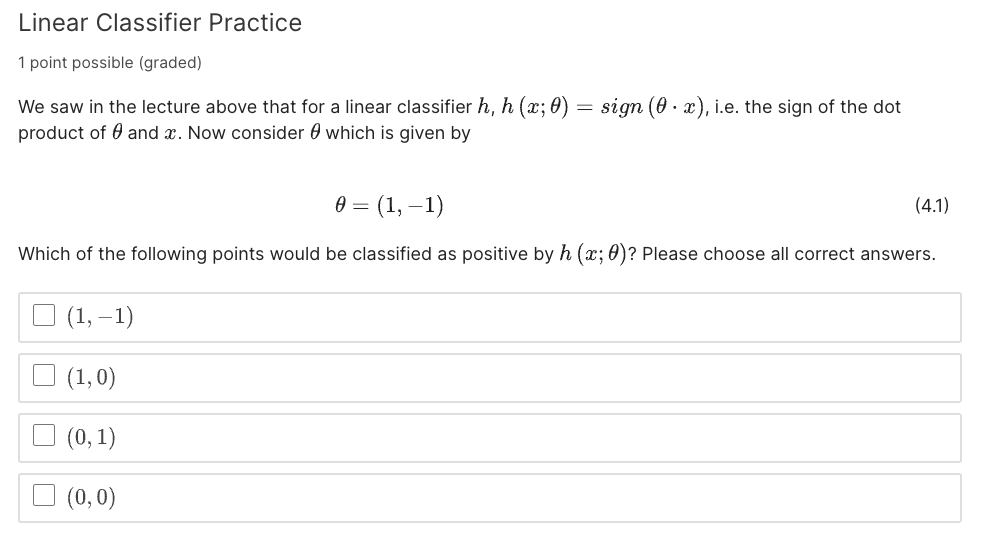
For a binary classification problem where the classes are labeled as -1 and 1, the decision rule can be written as:
Here, the “sign” function returns -1 if \(w.x + b < 0\), and 1 if \(w.x + b ≥ 0\).
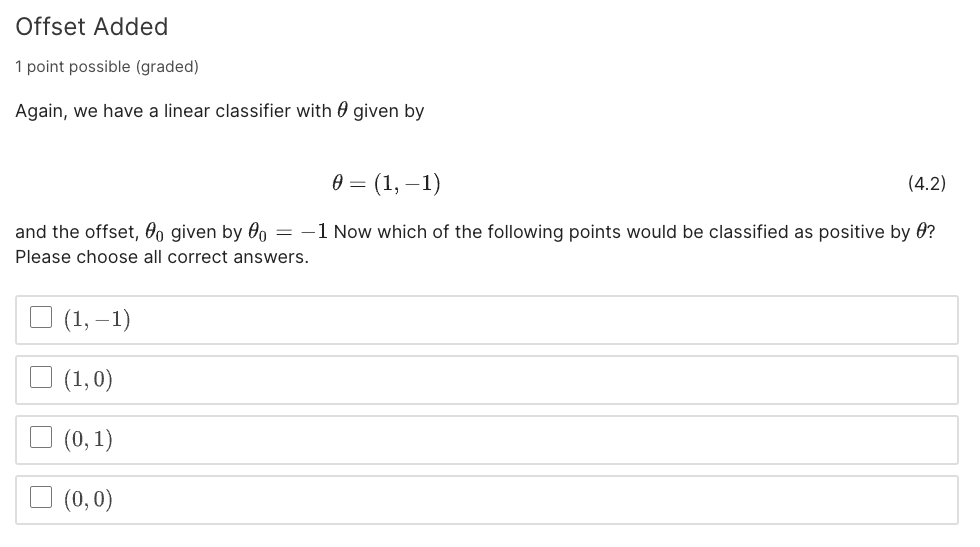
import numpy as np

"""
Linear Classifer solution
"""

# binary weights
theta = np.array([1,-1])
theta_offset = -1

# Define two vectors
x1 = np.array([1, -1])
x2 = np.array([1, 0])
x3 = np.array([0, 1])
x4 = np.array([0, 0])

# h(x, theta) = sign(dot(theta , x))
classifier = np.sign(np.dot(theta, x1))

# Without Offset
print("Classifer response for x1:", np.sign(np.dot(theta, x1)))
print("Classifer response for x2:", np.sign(np.dot(theta, x2)))
print("Classifer response for x3:", np.sign(np.dot(theta, x3)))
print("Classifer response for x4:", np.sign(np.dot(theta, x4)))

# With Offset
print("Classifer response with offset for x1:", np.sign(np.dot(theta, x1) + theta_offset))
print("Classifer response with offset for x2:", np.sign(np.dot(theta, x2) + theta_offset))
print("Classifer response with offset for x3:", np.sign(np.dot(theta, x3) + theta_offset))
print("Classifer response with offset for x4:", np.sign(np.dot(theta, x4) + theta_offset))
Classifer response for x1: 1
Classifer response for x2: 1
Classifer response for x3: -1
Classifer response for x4: 0
Classifer response with offset for x1: 1
Classifer response with offset for x2: 0
Classifer response with offset for x3: -1
Classifer response with offset for x4: -1
